Big-O Notation — Breakdown
If you’re like me when you first started to learn to program, you didn’t think much about efficiency. You just knew that your function or method accomplished a particular task, no matter how long it took. Over time though in your progression, you kept seeing things like ‘Big-O notation’, ‘time complexities’, ‘Asymptotic Analysis’. In this blog I’m gonna break down what all this means in a reasonable way (hopefully), so we can all better understand it.
Here’s a quick glossary to refer back to as you read through this blog. I figured it was easier to put all the definitions in one spot.
- Asymptotic analysis— of an algorithm refers to defining the mathematical boundation/framing of its run-time performance. Using asymptotic analysis, we can very well conclude the best case, average case, and worst case scenario of an algorithm.
- Big-O notation - is used in Computer Science to describe the performance or complexity of an algorithm. Big-O specifically describes the worst-case scenario, and can be used to describe the execution time (complexity) required or the space used (e.g. in memory or on disk) by an algorithm.
- Constant time - effectively means that an algorithm’s time complexity isn’t affected by the input size. Sometimes referred to as bounded time.
- Exponential time - these algorithms are costly. Exponential times increase dramatically in relation to the size of the input.
- Factorial time - these algorithms are even more costly then exponential algorithms.
- Linear time - this means the amount of work depends on the size of the input. Less efficient the bigger the input.
- Logarithmic time - narrows search by repeatedly halving the input until target value is found.
- N log2N - time involves applying a logarithmic algorithm N times.
- Quadratic time - algorithms of this type typically involve applying a linear algorithm N times.
Big-O or Big-0 ?
When I first heard the term ‘Big-O’, I wanted to know why it was called that. A little spiraling down the rabbit hole and a few internet searches later I understood a little bit more. First let’s clarify. It’s the letter O not the number 0. But why is it called Big-O in the first place? Because it’s a ‘Big’ ‘O’, get it? So what does the O stand for? ‘Order’, or ‘order of complexity’. This link give’s a little back history of what it means. It goes into how the O is actually an Omicron symbol which represents ‘order of’ and dates back to the late 1800’s. Ok enough mumbo jumbo history lesson. Just remember that Big-O notation is used to find the worst case scenario of the time it takes an algorithm to do it’s job.
Time Complexity
Time complexity basically means how long does an algorithm take to accomplish it’s task. Now I don’t mean you get your stop watch out and time your function till it finishes with a result. Here’s where Asymptotic Analysis comes into play. Asymptotic Analysis helps evaluate the performance of an algorithm based on the size of the input. So an algorithm’s time or space efficiency is measured as the input size grows.
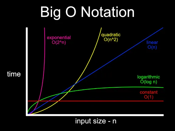
We’ve probably all seen a chart similar to this one. A quick reference for us showing common time complexities. Here’s a quick reference starting with the slowest growing function -
Notation and Name
- O(1) Constant time complexity
- O(log n) Logarithmic time complexity
- O(n) Linear time complexity
- O(n log n) n log n time complexity
- O(n²) Quadratic time complexity
- O(2^n) Exponential time complexity
- O(n!) Factorial time complexity
O(1) Constant Time
This is the best option. This algorithm time or (space) isn’t affected by the size of the input. It doesn’t matter. Also referred to as bounded time. An example of this is finding an indexed item from an array.
// Constant Timelet arr = [10, 4, 20, 2, 100, 5];
arr[4]; // => 100
O(log n) Logarithmic Time
The amount of work depends on the size of the input. Algorithms that successively cut the amount of data to be processed in half at each step typically fall into this category. Binary search algorithm falls within this category. But the array must be sorted for this to work.
// Logarithmic Time using Binary Searchlet arr = [1, 3, 4, 5, 6, 8, 9, 11, 12, 13, 15, 16, 17, 19, 20];function binarySearch(arr, value) {
    let left = 0,
        right = arr.length - 1;    while (left <= right) {
        let mid = left + Math.floor((right - left) / 2);
        if (arr[mid] === value) {
            return mid;
        } else if (arr[mid] < value) {
            left = mid + 1;
        } else {
            right = mid - 1;
        }
    }
    return -1;
}binarySearch(arr, 8); // => 5binarySearch(arr, 7); // => -1
O(n) Linear Time
The time to execute the algorithm is directly proportionate to the size of the input. Linear algorithms become terrible with an increasing input size. An example of a Linear algorithm is, what do you know, Linear Search Algorithm. This algorithm searches through an unsorted array looking for a value. Worse case scenario it has to check each individual value of the entire array to find the desired value or return that it couldn’t find the value.
// Linear Time using Linear Searchlet arr = [300, 2, 21, 6, 1000, 50, 450, 656, 23, 74, 33, 43, 211];function linearSearch(arr, value) {
    for (var i = 0; i < arr.length; i++) {
        if (arr[i] === value) {
            return i;
        }
    }
    return -1;
}linearSearch(arr, 211); // => 12linearSearch(arr, 10000); // => -1
O(N log2N) Time
Algorithms of this type typically will apply a logarithmic algorithm N times. Basically that’s it. An algorithm that will use O(log n) or Logarithmic a certain number of times to accomplish it’s task. The better sorting algorithms, such as Quicksort, Heapsort, and Mergesort, have O(N log2N) complexity. Let’s take a look at Mergesort.
// O(N log2N) Time using Merge Sortlet arr = [5, 6, 12, 4, 200, 56, 5, 18, 7];function mergeSort(arr) {
    if (arr.length === 1) {
        return arr;
    }    const mid = Math.floor(arr.length / 2);
    const left = arr.slice(0, mid);
    const right = arr.slice(mid);    return merge(mergeSort(left), mergeSort(right));
}function merge(left, right) {
    let result = [];
    let indexLeft = 0;
    let indexRight = 0;    while (indexLeft < left.length && indexRight < right.length) {
        if (left[indexLeft] < right[indexRight]) {
            result.push(left[indexLeft]);
            indexLeft++;
        } else {
            result.push(right[indexRight])
            indexRight++;
        }
    }
    return result.concat(left.slice(indexLeft))
                 .concat(right.slice(indexRight));
}mergeSort(arr); // => [ 4, 5, 5, 6, 7, 12, 18, 56, 200 ]
O(N²) Quadratic Time
Instead of calling a Logarithmic Algorithm n times. Quadratic calls a Linear Algorithm n number of times. Quadratic Algorithms involve nested iterations, such as nested for loops. The deeper a loop is nested can produce results such as O(N³) or O(N⁴). An example of an Quadratic Algorithm is insertion sort.
// Quadratic Time using Insertion Sortlet arr = [300, 2, 21, 6, 1000, 50, 450, 656, 23, 74, 33, 43, 211];function findMinAndRemove(arr) {
    let min = arr[0];
    let minIndex = 0;
    for (var i = 0; i < arr.length; i++) {
        if (arr[i] < min) {
            min = arr[i];
            minIndex = 1;
        }
    }
    arr.splice(minIndex, 1);
    return min;
}function insertionSort(arr) {
    let sortedArray = [];
    let min;
    while (arr.length !== 0) {
        min = findMinAndRemove(arr);
        sortedArray.push(min);
    }
    return sortedArray;
}insertionSort(arr); // => [ 2, 6, 6, 23, 23, 23, 23, 23, 33, 33, 43, 211, 300 ]
O(2^n) Exponential Time
These algorithms are costly. Exponential time increases dramatically with the size of the input. An example of Exponential time is a basic function for the Fibonacci sequence.
// Exponential Time using Fibonacci Sequencefunction fibonacci(position) {
    if (position < 3) return 1;
    else return fibonacci(position - 1) + fibonacci(position - 2);
}fibonacci(20); // => 6765
O(n!) Factorial Time
This is very very bad! You don’t see it too often. You know why? It’s very very bad! The Traveling Salesman problem is an example of factorial time.
Finally finished
As I wrap up this review of Big-O Notation I hope this gives you a little bit better understanding of how it works. Big-O really helps us understand the efficiency of our algorithms we write. If there is anything I left out or should add please leave a comment. Goodbye for now.